Small Network
What happens when you treat a neural network not as something to be trained, but as an agent in its own right? Not a model of a function, but a physical system with its own dynamics, producing temporal patterns that might, under the right conditions, sound like music?
This project began with a small spiking neural network, 256 threshold neurons wired together at random, and the question of whether evolutionary pressure could shape its output into something worth listening to. Over long series of experiments, the system evolved into a compositional engine that produced twelve pieces across three Japanese pentatonic scales: In-Sen, Iwato, and Kumoi. The raw MIDI output was then interpreted in Ableton Live, where timbre, texture, and spatialization gave the compositions their final voice.
The relationship between composition and interpretation here is worth dwelling on. John Cage’s chance-determined scores were often beautiful in performance, not because the I Ching produced great music, but because the performers brought their own sensitivity to the material. The compositions that came out of this network are similar. They have structure, repetition, surprise. But it’s the act of rendering them through specific instruments and effects that makes them feel alive.
The Network
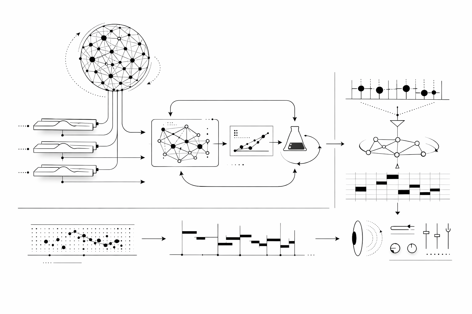
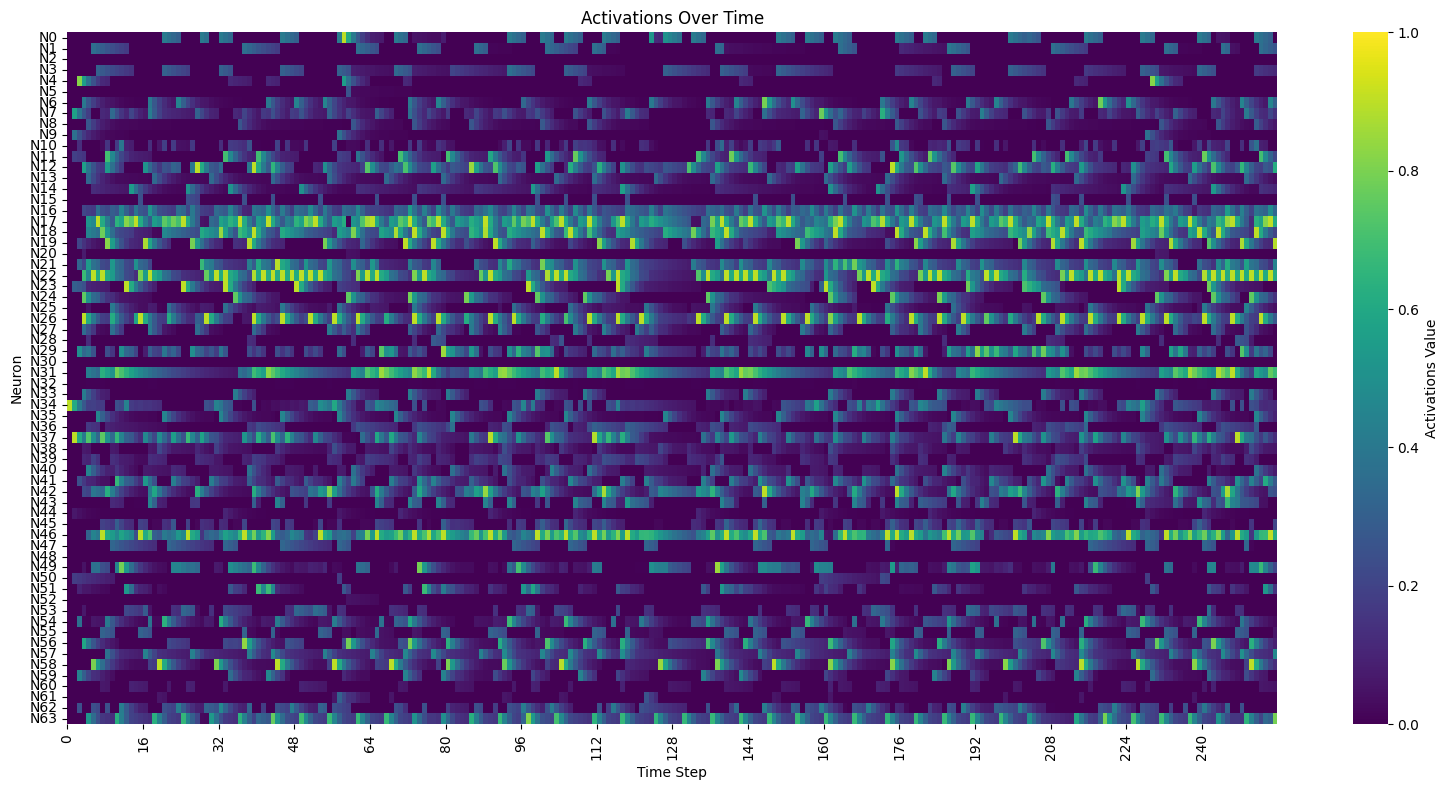
The architecture is deliberately primitive. Each neuron accumulates incoming activation, fires when it crosses a threshold, then goes quiet for a refractory period before it can fire again. Connections between neurons carry weights that can be excitatory or inhibitory. There is no training, no backpropagation, no gradient. The network just runs.
incoming = weights.T @ firing.astype(np.float64)
state.activations = state.activations * activation_leak + incoming
state.activations[state.refractory_counters > 0] = 0
state.firing = state.activations >= state.thresholds
This is structurally similar to what the reservoir computing literature calls the “liquid” in a liquid state machine: a recurrent, highly nonlinear dynamical system whose internal states are read out through a separate output layer. Wolfgang Maass introduced this idea in 2002, proposing that neural microcircuits are ideal “liquids” for computation because of the diversity of their elements and the variety of time constants in their interactions. The Sakana AI lab’s more recent Continuous Thought Machines paper takes a related approach, using neuron-level temporal processing and synchronization as a latent representation.
Our interest was narrower. We weren’t trying to solve a prediction task or classify inputs. We wanted the network to act as a sequencer, an autonomous system that produces temporal patterns with enough structure to be musical and enough unpredictability to be interesting. No external input, no driving signal. Just an initial stimulus and whatever the topology and weights produce from there.
The key parameters turned out to be the ones governing the network’s temporal behavior. Refractory periods, which determine how long a neuron stays silent after firing, have an outsized effect on rhythm. Activation leak, the rate at which accumulated potential decays, determines whether activity can sustain across longer silences or dies out. With a leak of 0.90 and a refractory period of 4 steps, only 66% of activation survives. Bump the leak to 0.98 and the network can hold tension across longer gaps.
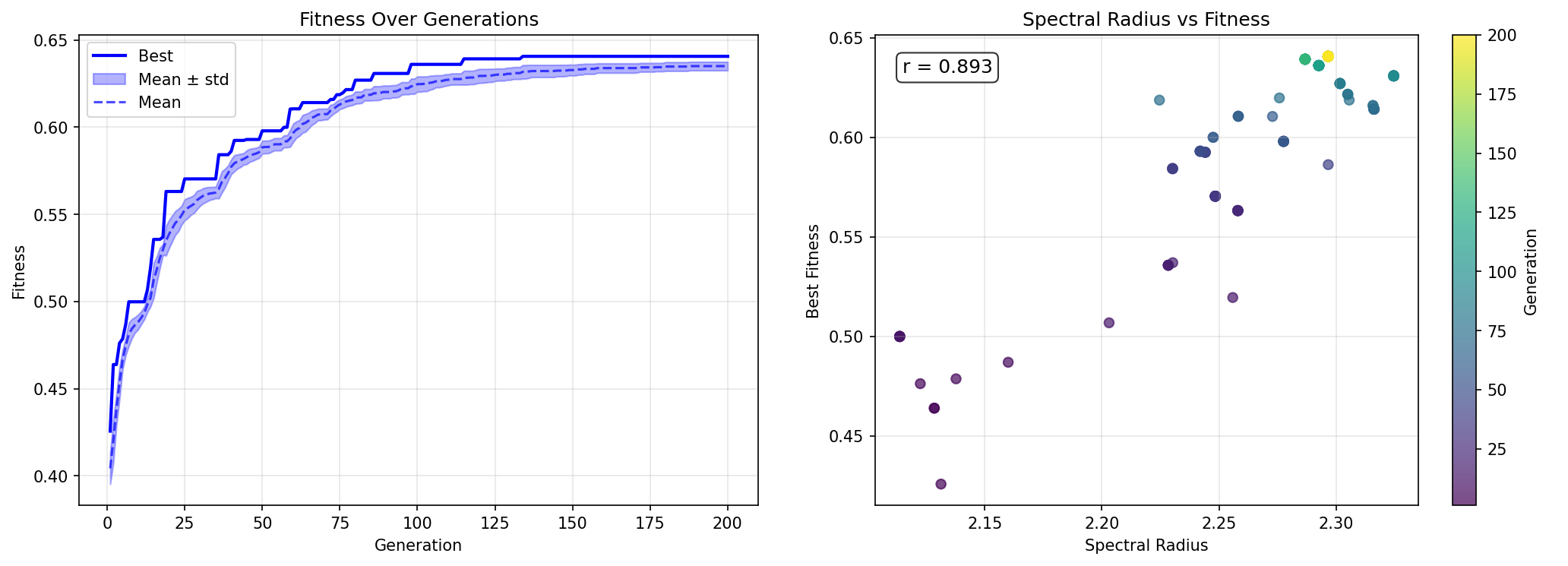
Spectral radius, a concept from Echo State Networks, captures the excitatory potential of the weight matrix. Too low and activity dies. Too high and the network saturates, every neuron firing every step. Chris Kiefer, in his work on Echo State Networks for musical instrument mapping, uses it as a kind of gain knob. We found that adding inhibitory connections was more effective than fine-tuning the spectral radius. Once inhibition was in the mix, the dynamics became far more varied, even without any exotic threshold schemes.
The Mapping Problem
A spiking neural network produces activation traces. Music requires notes with onset, duration, pitch, and volume. The gap between these two things is where most of the difficulty lies.
The first approach was direct: assign each neuron to a pitch, fire a note when activation crosses a threshold. This produces arpeggios. Fast, repetitive, all on the same time scale. These get dull rather quickly.
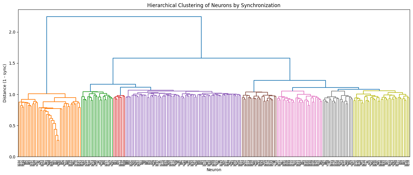
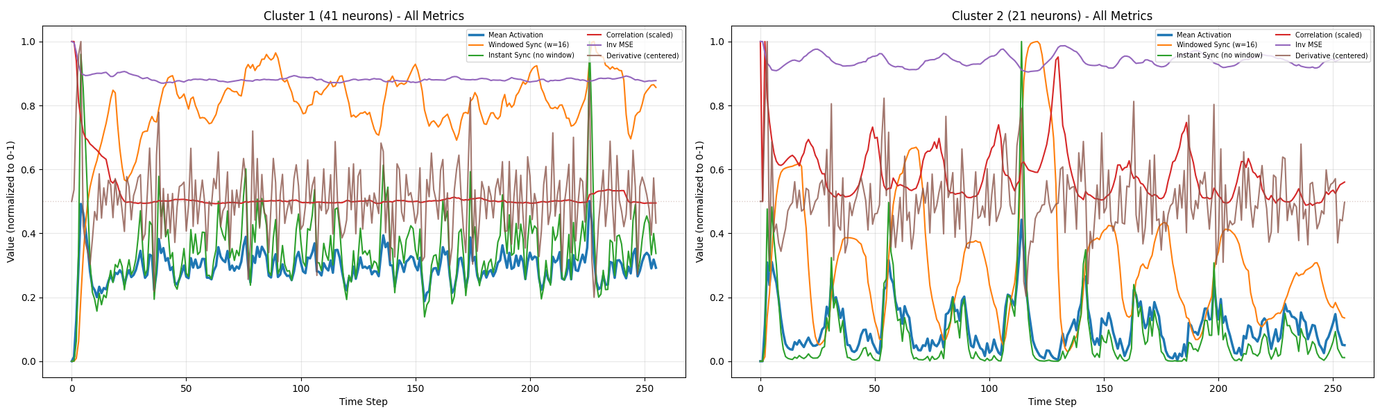
We tried clustering neurons by synchronization, following the method from the Continuous Thought Machines paper. Compute the dot product of neurons’ activation histories to find groups that fire together consistently. Map each cluster to a pitch. This was conceptually appealing but ran into a problem: activation, pitch, and volume all derive from the same signal. A loud note is a spiking note is a short note. Everything is correlated. Outputs become repetitive staccato.
An output layer approach worked better. Rather than clustering, create separate readout vectors, each connecting to the network through its own random weight pattern. Four readouts become four voices, each with its own weighted view of the network’s state. This is standard reservoir computing architecture: the reservoir (network) provides complex dynamics, the readout (output weights) extracts useful signals.
Two encoding schemes emerged from experimentation:
Pitch encoding gives each voice 12 outputs, one per chromatic pitch class. The highest output wins (argmax). Simple, direct, but the network has to discover scale structure on its own.
Motion encoding treats pitch as relative movement. Competing “up” and “down” forces with different interval weights determine how far the current pitch moves from the last one. The interval weights (1, 4, 7 semitones up; 1, 3, 8 semitones down) were chosen for their musical content: minor thirds, major thirds, fifths, octaves.
Both encodings use a fixed activation threshold rather than any adaptive scheme. This was a hard-won lesson. Adaptive thresholds, whether percentile-based or peak-relative, remove the network’s ability to control its own activity level. The evolution can’t learn to be sparse if the threshold always adjusts to guarantee a certain density.
Evolution
The evolutionary algorithm is a (μ+λ) strategy: maintain a population of μ parents, generate λ offspring through mutation, keep the best μ from the combined pool. No crossover. The literature and our own experiments confirmed that crossover tends to wreck neural networks, destroying the delicate balance between weights that produces coherent dynamics.
Fitness
The fitness function went through many iterations. The first attempt used eleven metrics borrowed from computational musicology, each with its own weight. This was too complex. The search space is already enormous, and competing objectives create Pareto frontiers that the algorithm can’t navigate.
We stripped it down to three components: modal consistency (do the notes fit a scale?), activity (is the network producing roughly the right density of notes?), and diversity (is each voice using a range of pitches, not just repeating one?).
To sanity-check the fitness function, we downloaded some ambient MIDI files, including Brian Eno’s Music for Airports, and ran them through the evaluator as a baseline. After 37 generations our best network scored roughly on par with the ambient comparison set. We had already surpassed Music for Airports. Either the fitness function had failed us, or we had accidentally evolved Brian Eno with 256 neurons.
Activity scoring was tricky. A simple minimum threshold rewards spam. The fix was a Gaussian target function in log-space:
ratio = note_density / target_note_density
score = np.exp(-0.5 * (np.log(ratio))**2)
Perfect score at the target density, symmetric penalty for overshooting and undershooting.
Diversity had its own failure mode. The global metric could be gamed: four voices each repeating a single note, but different notes across voices, yields decent entropy. The fix was per-voice diversity, taking the minimum across voices.
Further refinements to fitness are discussed in the Gravity section below.
What Evolution Taught Us
The first surprise was that evolution works at all. Small mutations to the weight matrix of a chaotic dynamical system tend to produce wildly different behavior. The sensitivity of spiking networks to parameter changes means most mutations are destructive. Early runs showed random search competing with mutation until we brought the mutation scale down to 0.001.
The second surprise was how quickly the population converges. Lineage tracking revealed that one lineage typically dominates within five generations. With 20 parents and 100 offspring, selection pressure is intense. We tried speciation, fitness sharing, island models. None helped much. The problem wasn’t population diversity but the fitness landscape itself.
The third surprise was that network physics matters more than evolutionary strategy. Changing the activation leak from 0.90 to 0.98 had more impact than any clever mutation scheme. Refractory period distribution, initial sparsity, weight scale: these hyperparameters define the space evolution searches through, and they’re more determinative than anything the search does within that space.
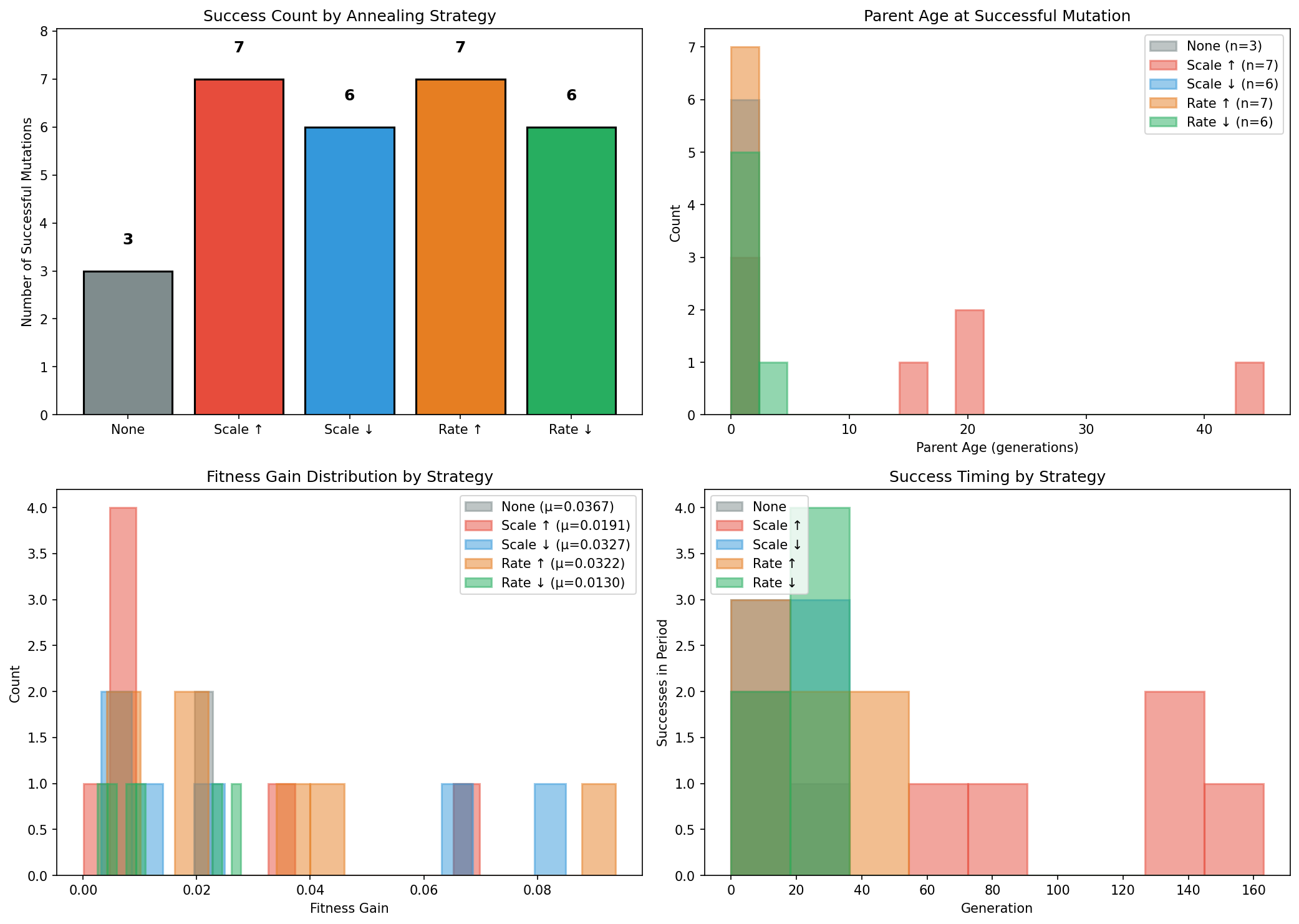
We did try several evolutionary refinements. Mutation annealing based on parent age: if a parent hasn’t been improved on in many generations, increase the mutation scale. The population was split into five groups, each with a different annealing strategy, to compare directly. More aggressive annealing helped somewhat.
Topology evolution was another front. Originally, only existing non-zero weights could be mutated. Zero weights stayed zero forever, locking the connectivity pattern at initialization. Removing this mask allowed new connections to form. But then a new problem emerged: mutations can only add connections (a zero weight plus gaussian noise becomes non-zero), never remove them (a non-zero weight won’t randomly land on exactly zero). Networks become monotonically denser.
The solution was a functional threshold: weights below 0.05 are treated as zero during simulation, even if their stored value is nonzero. Weak connections are effectively pruned. Selection can push the network toward either sparse, strong connections or dense, weak ones.
effective_weights = np.where(
    np.abs(state.network_weights) >= state.weight_threshold,
    state.network_weights, 0
)
But this threshold also created a dead zone. With initial sparsity at 10%, 90% of weights start at zero. Mutation scale of 0.001 means a zero weight becomes roughly 0.001 after mutation, still far below the 0.05 threshold. It would take about fifty aligned mutations to cross that barrier. The topology was effectively frozen.
Vectorization
A practical note. The original simulation used nested Python loops: 256 neurons × 256 neurons × 128 timesteps = ~8 million loop iterations per evaluation. Each generation took about 24 seconds. Replacing the inner loops with a single NumPy matrix multiply dropped simulation time from 233ms to 4ms, a 58x speedup. Full generation time went from 24 seconds to 1.2 seconds. This made iteration possible.
Baking the Scale In
The breakthrough that made the final pieces possible was a conceptual shift: stop trying to evolve tonality and just give it to the network for free.
With 12 chromatic outputs, modality (staying in a scale) and diversity (using many pitches) are directly at odds. Every additional note is another chance for an out-of-scale error. The fitness function was fighting itself.
The fix was to reduce the output layer from 12 to 5, one per note of a pentatonic scale. Every note the network can produce is in-scale by construction. Modality is guaranteed, so it drops out of the fitness function entirely:
IN_SEN_SCALE = [0, 1, 5, 7, 10]  # C, Db, F, G, Bb
DEFAULT_N_OUTPUTS_PER_READOUT = len(IN_SEN_SCALE)
To change the scale, edit one line. The same network architecture and evolution code produced pieces in In-Sen, Iwato, and Kumoi by simply swapping the scale definition.
This also made differential evolution viable. Standard mutation adds random noise: child = parent + gaussian. Differential evolution adds a structured delta: child = parent + F * (better - worse). The difference vector between two parents of different fitness encodes which weights matter and which direction to push them. It’s self-scaling: when the population is diverse (early generations), the deltas are large. As parents converge, the deltas shrink automatically.
new_weights = clip(self.weights + F * (better.weights - worse.weights), -1, 1)The combination of pentatonic encoding and differential evolution produced a dramatic speedup. Fitness jumped to ~0.8 in 2 generations instead of 48. The pentatonic encoding removed a bad objective. Differential evolution provided structured search in the remaining space.
Gravity
The next challenge was tonal gravity: making the music feel rooted in the scale’s characteristic intervals without simply weighting the root note more heavily. Japanese pentatonic music derives its identity from specific melodic motions, the half-step pull between C and Db in In-Sen, the dual semitone poles of C↔Db and F↔Gb in Iwato, the D↔Eb color against the structural C-G fifth in Kumoi.
We defined target transition matrices for each scale encoding these characteristic motions, then scored how well each voice’s transitions matched the target. The first implementation graded each transition individually: “given you’re on C, did you go somewhere good?” This was immediately exploited. Every voice converged to oscillating between C and Db, scoring 0.94 on tonal gravity while sounding terrible. The metric couldn’t see the problem because it only graded transitions that actually occurred, never noticing that 18 of the 20 possible transition types were absent.
The fix was to compare the full distribution of transitions against the target using KL divergence. Instead of asking “was each move good?” it asks “is the overall mix of moves right?” An oscillator now concentrates 100% of its probability on 2 of 20 transition types while the target expects those 18 missing types to account for 83% of all movement. The KL divergence explodes and the score drops to near zero.
This also resolved a deeper conflict: the old pitch entropy metric (rewarding uniform note usage) was fundamentally at odds with tonal gravity (rewarding preferred transitions). The joint distribution approach subsumes both, the target already specifies which transitions should be common and which rare, implicitly defining the right pitch distribution. The final composite became activity × tonal gravity × repetition, where tonal gravity handles both idiom and variety, and the n-gram repetition penalty catches sequential monotony that distributional metrics can’t see.
The Pieces
The final engine ran twelve evolution sessions, four per scale. Each session produced a best-of-generation MIDI file: four voices of pentatonic melodies, each with its own rhythmic character, emerging from the same underlying neural dynamics. The three scales used were In-Sen (C, Db, F, G, Bb), Iwato (C, Db, F, Gb, Bb), and Kumoi (C, D, Eb, G, A).
The raw MIDI is sparse and rhythmically uneven. The network’s natural dynamics produce bursts of activity separated by lulls, which fits well with the Japanese pentatonic scales and a musical tradition that values intervals of silence.
These are still scores, not recordings. In Ableton, each voice was assigned an instrument and processed through effects chains that give the composition its sonic identity. Reverb, delay, saturation, filtering. The composition determines what happens when, but the interpretation determines what it sounds like and how it feels.
Some of Cage’s chance-determined music was enjoyable because of what the performers brought to it. Even though the compositions might have been completely chance-determined, the interpretation gave them a human quality, gave them meaning. These neural network compositions are similar. They have internal logic, repetition with variation, moments where voices converge and diverge. But they need a human ear to decide what weight to give each voice, what texture, what space.
What Was Learned
The reservoir metaphor works. Treating a spiking neural network as an autonomous dynamical system, with readout layers extracting useful signals, is a viable approach to generative composition. The architecture is structurally identical to an Echo State Network running in generative mode, with evolution replacing gradient-based training of the readout.
The network is mostly defined by its physics. Activation leak, refractory periods, sparsity, weight scale. These parameters set the boundaries of what evolution can discover. Most of the interesting musical properties come from getting these right, not from clever evolutionary strategies.
Encoding is everything. The choice of how to map network activations to musical events has more impact than any other design decision. Baking the scale into the encoding, rather than trying to evolve scale adherence, was a vital change in the project.
Evolution is a blunt instrument for neural networks. The sensitivity of spiking dynamics to small parameter changes makes gradient-free optimization difficult. Differential evolution helps by providing structured mutations. But the core challenge remains: after early convergence, both gaussian and differential mutations are too small to explore new regions of the landscape.
Simple is good. The final system has 256 neurons, 5 outputs per voice, 3 voices, and a three-component fitness function (activity × tonal gravity × repetitive penalty). Every attempt to add complexity, more metrics, more outputs, adaptive thresholds, speciation, ended up hurting more than helping.
What’s Next
The weight threshold dead zone remains unsolved. Networks can’t grow new strong connections because mutations are too small to cross the functional threshold. CMA-ES, which learns the full covariance structure of good mutations, might help.
There’s also the question of temporal structure. These compositions have local coherence but no large-scale form. No development, no arc. This is fine for ambient music, where stasis is a feature. But for other contexts, some mechanism for long-range structure would be needed. Perhaps nested networks at different time scales, or some external clock that modulates the network’s parameters over time.
The broader project, what we’ve been calling Flow Control, continues. The counting automata were one probe. These spiking networks are another. The underlying question is the same: what happens when computation handles the notes, and human attention focuses on everything else?