The Strange Agency

Building upon some techniques from a previous post, here we continue guiding Stable Diffusion with audio spectra.

Music: Claus Muzak

Process

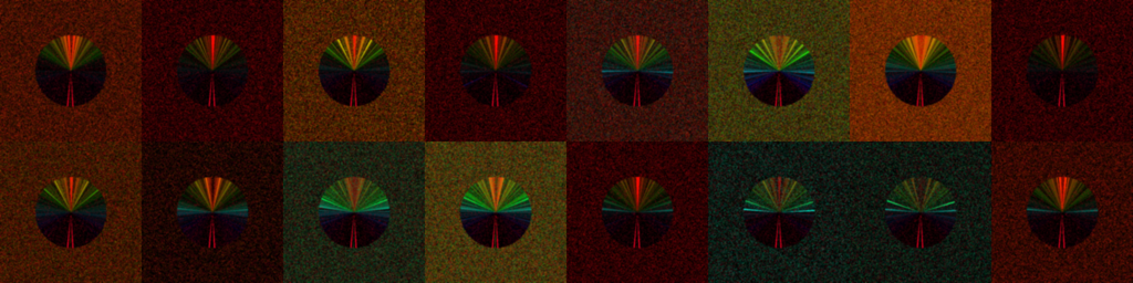
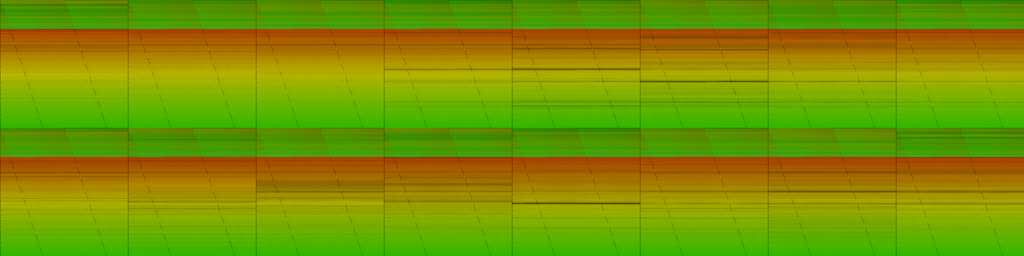
Starting with a blurred noise field as before, we then render the audio spectrum using pie slices. Of course this is not a typical way to render a spectrum, but it is also nothing particularly exotic. The code for a half pie (or one π) looks something like this:

draw = ImageDraw.Draw(im)
draw.pieslice(
    pos + size,
    i * angle_step - 90,
    (i + 1) * angle_step - 90,
    fill=color,
)

The results for the first few frames follow.

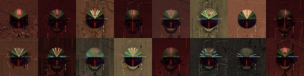
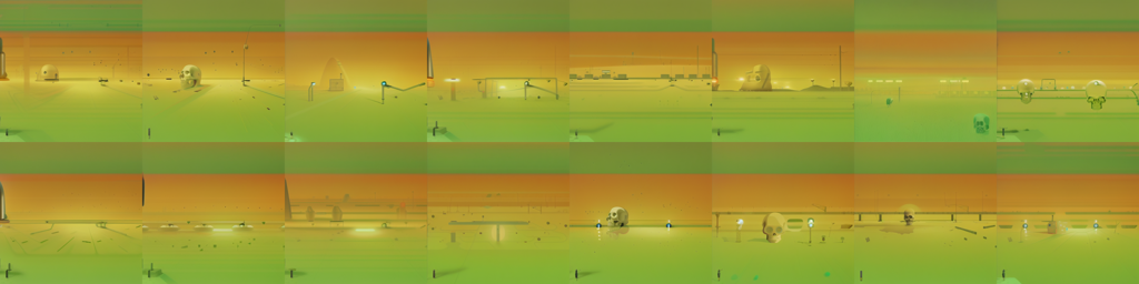
Using this to guide Stable Diffusion with some prompts about gas masks and helmets, we get a pleasant array of futuristic imagery, with a fanciful twist on the spectra above.

Desaturating the images also makes for some nice effects.

im = im.filter(ImageFilter.GaussianBlur(radius=2))
im = im.convert('L')  # desaturate
# im = ImageOps.invert(im)  # not using this, but fun to play with
im = ImageOps.autocontrast(im)
# im = ImageOps.equalize(im)  # cool, but probably too much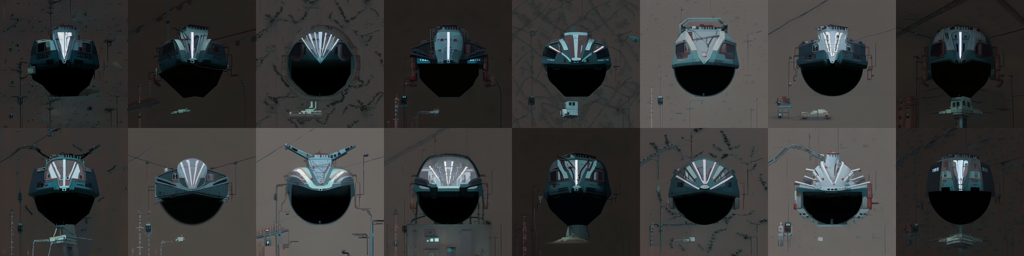

Drawing images in Python is not the best experience, so we also output a CSV of the frequency bins.

import math
from scipy.fft import rfft, rfftfreq

# similar to the way we created images, skipping some setup, we chop the audio and extract frequency content

for c in range(n_chunks):
sample_start = int(c * n_chunk_samples)
    sample_end = int(sample_start + n_chunk_samples)
    signal = signal_original[sample_start:sample_end]

    n_samples = sample_end - sample_start
    seconds = n_samples / float(sample_rate)

    n_channels = len(signal.shape)
    if n_channels == 2:
        signal = signal.sum(axis=1) / 2

    signal = np.divide(signal, 2**16)  # assuming 16 bit WAV here

    n_window_samples = math.floor(window_size * sample_rate)
    amps = rfft(signal, n_window_samples)
    amps = np.absolute(amps)
    freqs = rfftfreq(n_window_samples, 1 / sample_rate)

    indices = np.logspace(1, math.log(n_window_samples / 2, 10), num=256).astype(int)
    text_amps = np.take(amps, indices)
    texts.append(text_amps)

# but later write this to a file
import csv

with open("funky_out.csv", "w", newline="") as file:
    writer = csv.writer(file)
    writer.writerows(texts)

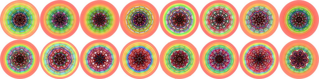
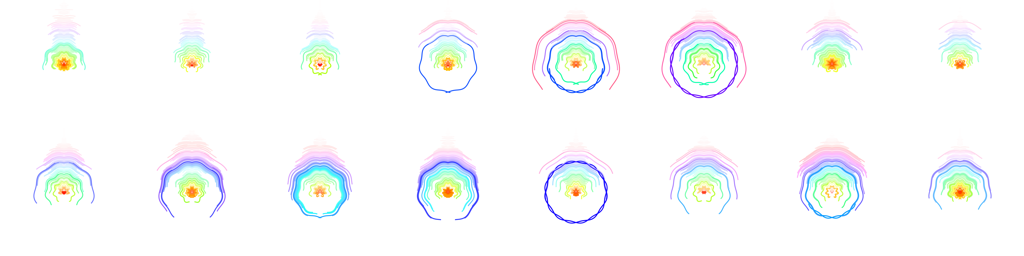
We can then import the CSV into a P5.js sketch to more quickly iterate on a variety of renderings.

Polar coordinates are always fun, so let’s try rendering with those.

function draw() {
    let frame = (frameCount - 1) % totalFrames;
    let step = size / totalBins;
    row = table.getRow(frame);

    translate(width / 2, height / 2);
    background(255);

    let n = 0;
    for (let i = 0; i < totalBins; i++) {
        let m = row.get(i);

        let c = color(i * 4, m * 2, 100);
        fill(c);

        for (let t = 0; t < m * 4; t++) {
            let theta = t - 90;
            let rho = i * 2 + sin(t * 8) * 4;

            // polar to cartesian
            let x = rho * cos(theta);
            let y = rho * sin(theta);

            circle(x, y, step);

            theta = 180 - theta;
            x = rho * cos(theta);
            y = rho * sin(theta);

            circle(x, y, step);
        }
    }
}

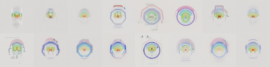
Finally, rendering the audio as circles yields the video at the top of this page.