Automatic Music Videos
In this post we will look at generating an audio spectrum and using that to feed a diffusion pipeline, with the aim of automatically generating a music video.
As we are focusing on ffmpeg and the audio spectrum, we will mostly be using default diffusion parameters. See our other blog posts for deeper dives into these.
The insanely capable ffmpeg can be used to create audio spectrum visualizations of input audio. With the right commands, ffmpeg can actually do your dishes and walk your dog, but for today we shall stick to videos. There are a few different visualization options, and here we will choose the CQT visualizer, as it is tuned to the musically salient aspects of the input signal.
For more details, have a look at the showcqt filter.
Convert input audio to a video output representing frequency spectrum logarithmically using Brown-Puckette constant Q transform algorithm with direct frequency domain coefficient calculation (but the transform itself is not really constant Q, instead the Q factor is actually variable/clamped), with musical tone scale, from E0 to D#10.
Below we use the filter to generate a spectrum video, rotate it 90º, mirror it, and dump the resulting frames into a folder.
# extract spectrum
ffmpeg -i input.wav -filter_complex \
"[0:a]showcqt=s=512x512:r=30:axis=0,format=yuv420p[v]" \
-map "[v]" -map 0:a cqt.mp4
# rotate 90º
ffmpeg -i cqt.mp4 -vf "transpose=2" cqt_cc.mp4
# mirror
ffmpeg -i cqt_cc.mp4 -vf "crop=iw/2:ih:0:0,split[left][tmp];[tmp]hflip[right];[left][right] hstack" cqt_cc_mirr.mp4
# make a folder for PNGs
mkdir cqt
# turn mirrored video into frames
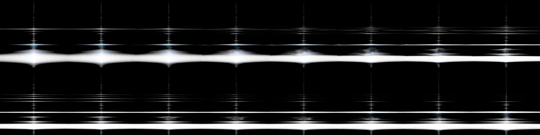
ffmpeg -i cqt_cc_mirr.mp4 cqt/$filename%04d.pngThe final mirrored output looks like this.
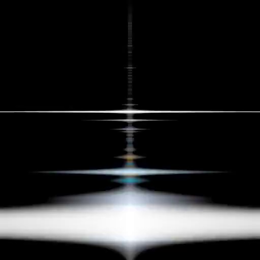
And below are the first 16 frames.
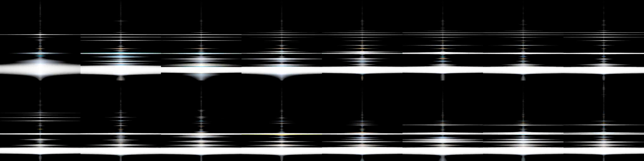
Spectrum, all frames
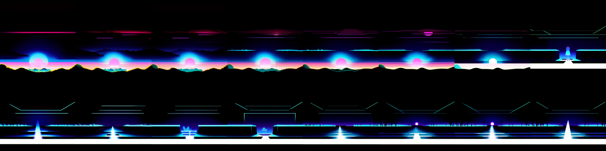
You can immediately batch this into an img2img pipeline of your choice, but looking at the above we see that there is a lot of variation between frames. When we run the spectrum frames through our diffusion model, we do see some coherence, but there is too much variability for smooth animation.
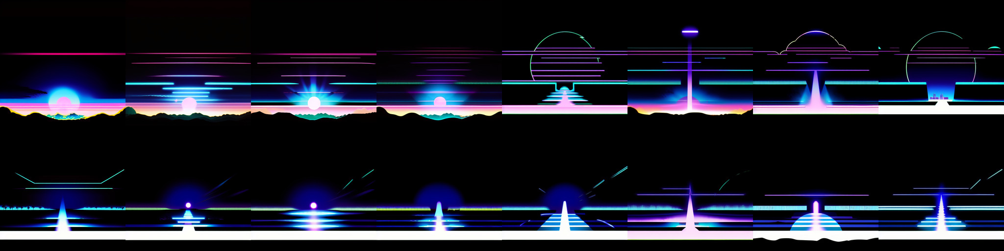
Spectrum, all frames diffused
One option might be to use ControlNet, subsampling control frames for less variability. We could also try outputting the spectrum using different framerate,tlength, or count settings. In this post we will try subsampling the frame output and interpolating between frames.
The final command outputs 635 frames. Our input audio is 21 seconds long, which comes to 630 frames at 30 fps. Apparently ffmpeg prefers 30.2380952381 fps. When the scientist in us goes for a smoke break, let’s fudge this further toward a greater numeric pleasure. Pretending we have 640 frames, we can do some pleasant math. The audio piece here is 4 bars long, and we mostly care about the spectrum at key moments, which likely fall on even note divisions. This is electronic music after all.
Looking at just sixteenth notes would require us to sample every 10th frame, 640/(4*16). However the interpolators we tend to use work in powers of two, as they double, quadruple, etc. the frame count. If we have every 10th frame, we will not be able to get back to our original frame rate. If we grab twentieth notes instead, 640/(4*20), we are using every 8th frame.
We can script against an API grabbing every 8th frame, but here we will just quickly prep a folder for batch processing.
mkdir cqt_8 && cp cqt/{0001..0635..8}.png cqt_8/Looking briefly at sampling every 8 vs 10 frames, we can see that the sets are not totally disjoint. This means that some of our samples will still fall on the musical sixteenth notes, where interesting transients occur.
# counting by 8
0001, 0009, 0017, 0025, 0033, 0041, 0049, 0057, 0065, 0073, 0081 ...

# counting by 10
0001, 0011, 0021, 0031, 0041, 0051, 0061, 0071, 0081 ...
In order to blend between the spectral samples, we will use our slightly-modified fork of FLAVR, as it can output still images. (Note that FLAVR apparently ignores the first and last frame, so we duplicate those to pad our input).
We will perform a 4x interpolation as well as an 8x. Perhaps we can 2x the 4x version after diffusion for a smoother result? For comparison, we also diffuse every 8th frame and interpolate the diffused results. In sum, we try subsampling and interpolating the spectrum and diffusing the result, subsampling and diffusing the spectrum and then interpolating the diffused result, and a bit of both.
python ./interpolate.py --is_folder --save_files --input_video "$INPUT_FOLDER" --factor 4 --load_model ../FLAVR_4x.pth

python ./interpolate.py --is_folder --save_files --input_video "$INPUT_FOLDER" --factor 8 --load_model ../FLAVR_8x.pth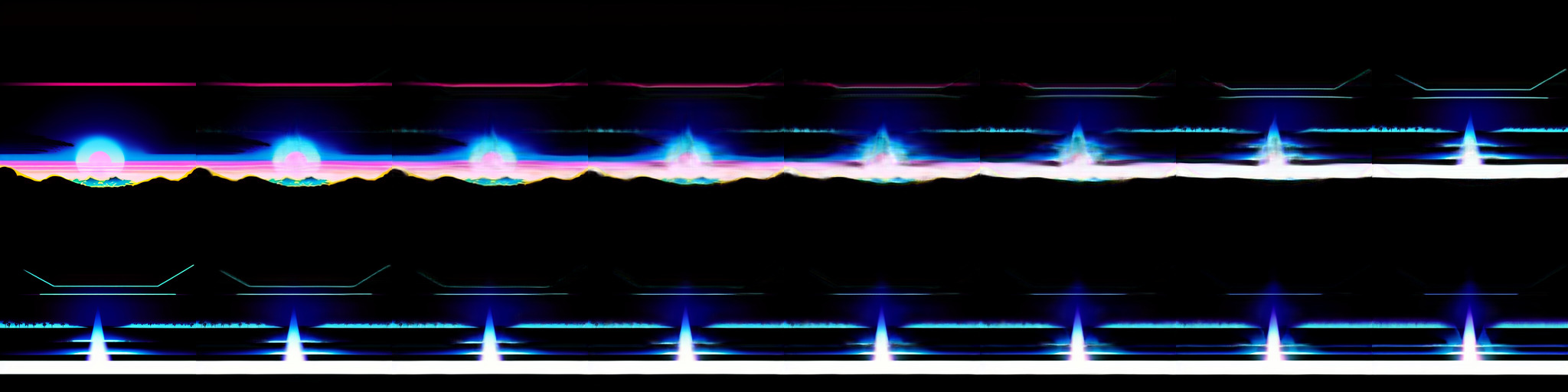
Every 8 frames, Diffused, Interpolated 8x
Sampled every 8 frames, Interpolated 8x
Every 8 frames, Interpolated 8x, Diffused
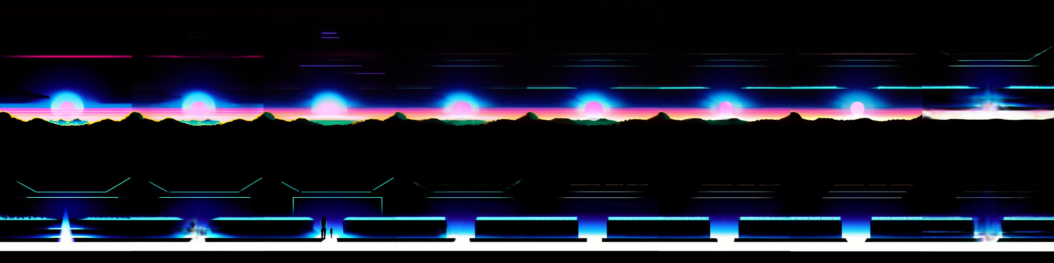
Every 8 frames, Interpolated 4x, Diffused, Interpolated 2x
We need a couple more ffmpeg command to tie all of this together, creating a video from still frames, and adding the original sound. The above process created many variations, but let’s assume the output we like is in a folder named output.
# create video from still frames
ffmpeg -framerate 30 -pattern_type glob -i 'output/*.png' -c:v libx264 -pix_fmt yuv420p output.mp4

# add audio to video
ffmpeg -i output.mp4  -i input.wav -map 0:v -map 1:a -c:v copy -shortest output_final.mp4
We post the results below. The hybrid process which interpolates before and after diffusion seems to give us the best audio response versus smoothness.
Interpolating the spectrum images does smooth out the video slightly, but the result is still very jittery. A nice feature is that the 8 frame rhythm of the interpolation is obscured by the frantic result.
The last option, interpolating the diffused images, is very smooth and does indeed follow the audio, but the 8 frame interpolation rhythm visually dominates the video.